Throughlines: Tracing Data With Field-level Lineage, Part 2
In Part 1 of Throughlines: Tracing Data With Field-level Lineage, we discussed how lineage was a natural extension of parsing SQL using our common definition model, as well as use cases for lineage. In this Part 2, we will cover more technical details about how we go from SQL to lineage.
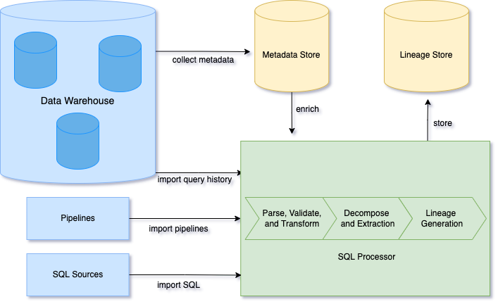
Single Origin requires a connection to your data warehouse that we use to collect and store metadata. This metadata helps us understand what tables exist in your warehouse. Then, when you import SQL queries, a SQL Processor extracts lineage information and keeps it in a time-series lineage store. This lineage store helps us understand what and how tables and fields are related. We can generate field-level lineage by combining the metadata and the lineage store.
Metadata Store
Single Origin connects to the data warehouse to collect metadata about the state of your datasets. We only collect necessary metadata to minimize cost. Once a connector is set up, our workflow starts collecting metadata such as the table schemas, descriptions, ownership, and usage information.
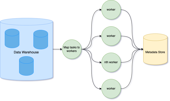
To collect a large amount of metadata, we build a metadata store that can be scalable and extensible. The metadata store powers features such as data discovery and authoring.
Each metadata is considered to be an attribute of the entity that can continually be updated or expanded upon.
Example of how metadata attributes are stored for the order_items column.
For a more accurate field-level lineage, we leverage column names and data types in our SQL processing. When ingesting column information into Single Origin, we map them into our standardized data types.
Standardized Data Types
Standardizing data types in the metadata store allows us to extend SQL processing to other data warehouses and manage data entities in a multi-cloud environment. The SQL Processor will need to only interface with one metadata store rather than every data warehouse implementation.
Data types are mapped to Single Origin standardized data types.
Data types from different sources may have different names for the type. In some cases, one type may not be supported in another data source. For example, Snowflake has semi-structure data support rather than a data type with struct fields explicitly defined like in BigQuery. Standardization of the data types inside our metadata store allows our downstream data systems to be agnostic toward the source of the metadata.
The metadata store is the foundation for accurate field-level lineage. Before we go into SQL Processing, let’s take a look at how we store the lineage.
Lineage Store
The Lineage Store records entity relationships and how they are derived. Once a SQL query has been processed, the derived lineage is saved in the Lineage Store for operational queries. In each lineage event, we store the context of how the relationship was created.
Lineage Context
Each lineage event has additional information such as the SQL transformation, what operation was used, and the time it occurred. This allows users to quickly understand how field-level data was transformed and used over time.
Example of a lineage with SQL transformation as context and the type of lineage, which we will go into more detail in the later section.
As shown in the table, the lineage store is composed of time-series data about every SQL query that went through the SQL processor.
Time-series Lineage
Lineage is an active system that is updated continuously. Data pipelines and table schemas are frequently changed by Data Engineers and Data Scientists; lineage information that was captured a day ago may no longer be valid. To ensure we can capture these changes, we maintain a time-series system in order to reflect the most accurate lineage information.
When a new create or update query is detected, the lineage store is updated. Our API queries the last 30 days of lineage events by default, but we also provide an option to get the latest lineage information beyond the default time window.
Lineage data powers various workflows in Single Origin, from detecting changes to rendering the interactive graph on the UI. We have integrated field-level lineage into the core of Single Origin by detecting changes that can impact downstream consumers.
Before the lineage events can be ingested into the time-series lineage store, each SQL must be processed to derive the field-level lineage.
Turning SQL into Lineage
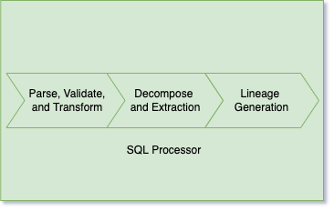
The above architecture graph demonstrates the three steps required to extract a lineage graph from a given SQL query.
- Parsing, validation, and transformation
- Decomposing and extracting
- Lineage generation
Parse, Validation, and Transformation
Single Origin parses SQL into AST (abstract syntax tree) based on Calcite which validates the AST with the standardized schema in the metadata store. During the validation process, the scope of each syntax node is derived and verified, ensuring a higher level of accuracy than parsing alone. When two or more nodes have the same name, the correct context for each is attached to the nodes by the validator. Additionally, if it is unclear which dataset a column is coming from, the validator can derive and extend the node's source prefix. With the correct context and source prefix, the underlying source for any node can be easily identified.
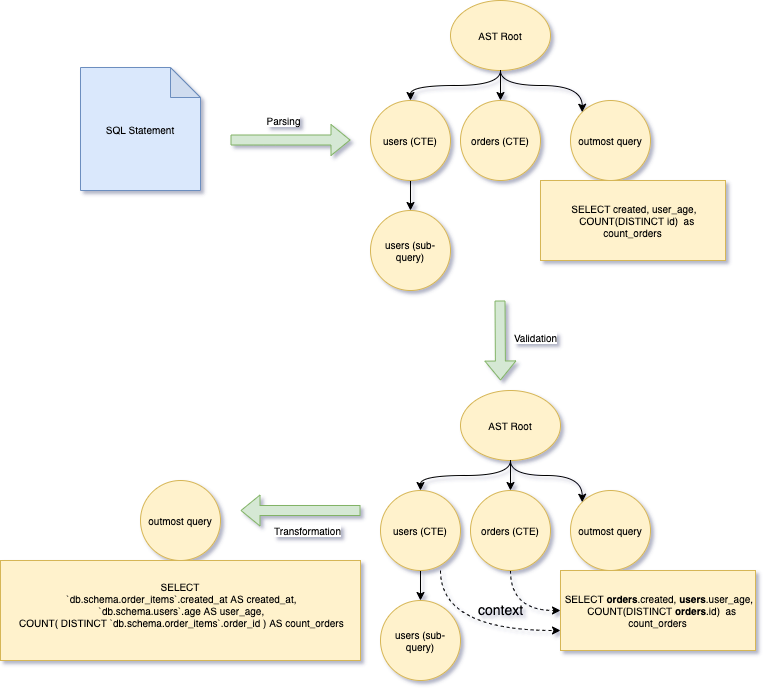
For example, the following SQL statement has two sub-queries with the name users, but they have different exposed columns. For the outermost query, Calcite knows the users pointing to the with clause item users with user_id and user_age. The outermost query selection items user_age and created_at don’t have a prefix to tell where they are from, but Calcite extends them as users.user_age and orders.created_at during the validation process.
CREATE TABLE
 `db.schema.user_order` AS (
 WITH
   users AS (
   SELECT
     id AS user_id,
     age AS user_age
   FROM (
     SELECT
       *
     FROM
       `db.schema.users` ) AS users ),
   orders AS (
   SELECT
     user_id,
     created_at AS created,
     order_id AS id
   FROM
     `db.schema.order_items`
   WHERE
     status = 'Returned'
     AND created_at >= '2022-01-01' )
 SELECT
   created,
   user_age,
   COUNT(DISTINCT id) AS count_orders
 FROM
   users
 JOIN
   orders
 ON
   users.user_id = orders.user_id
 GROUP BY
   1,
   2 )
For brevity, we replace the concrete project and dataset name with db.schema and skip the prefix in the examples.
After the parsing and validation, we leverage the relational operator properties to transform the original SQL AST to another canonical form AST where all the expressions are directly based on the underlying physical table. For the above query, the outmost transformed query is shown as the following statement.
Parsing, validation, and transformation are essential parts of lineage generation. Parsing the SQL statement into an AST allows for efficient traversal to extract the desired information. Validation ensures each AST node has the correct meaning (where it's from, what it's used for, and the like). Without validation, nodes become difficult to discern between, especially for nodes with the same name and node type. This would lead to an inaccurate lineage, where nodes may point to the wrong node, or where some edges may not be ascertainable. Lastly, the transformation from the original AST to a canonical AST eliminates the effect of alias naming and nested query structures, basing the lineage on the underlying physical datasets.
CREATE TABLE
 `db.schema.user_order` AS (
SELECT
 `db.schema.order_items`.created_at AS created_at,
 `db.schema.users`.age AS user_age,
 COUNT( DISTINCT `db.schema.order_items`.order_id ) AS count_orders
FROM
 `db.schema.users`
JOIN
 `db.schema.order_items`
ON
 `db.schema.users`.id = `db.schema.order_items`.user_id
WHERE
 `db.schema.order_items`.status = 'Returned'
 AND `db.schema.order_items`.created_at >= '2022-01-01'
GROUP BY
 `db.schema.order_items`.created_at,
 `db.schema.users`.age)
Decomposing and Extraction
During the decomposition process, it breaks the transformed SQL AST into source, selection items, where clause, and group by. All these decomposed items are used later for lineage generation. It generates the following items:
Lineage Generation
Given the above generated items, we first derive the schema of the target table based on the validated AST together with the standardized type information from the metadata store.
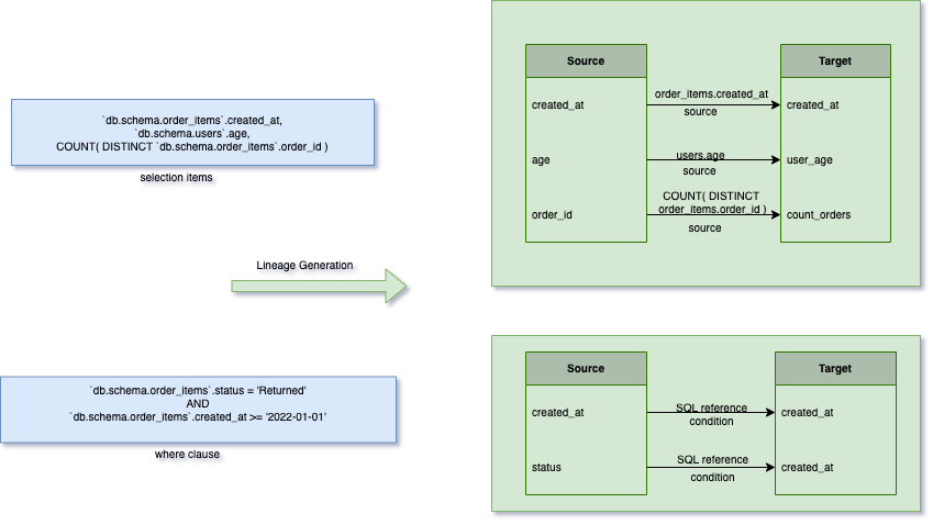
After the schema deriving, it processes all the selection items and generates the lineage edges for the corresponding field in the target table.
Finally, since the where clause affects the data in the target table, we process the where clause to derive the condition lineage. The condition lineage links the destination field with the where clause-related fields, so data operators can quickly recover the original SQL statement and understand how it affects the value of the destination field. The following table demonstrates the condition lineages for the destination field created_at. The same lineage edges are generated for the other two target nodes too.
Entity Lineage
In Part 1, we talked about breaking down the SQL into data entities, views, and dimensions and demonstrated the relationship between those entities. The relation is derived by the same process described above. For the above example, if we import it to generate data entities, views, and dimensions, it will generate the following view, data entity, and dimensions.
During the importing process, we generate the view fields for the view to represent its schema. Since the above view selects all columns from those two joined tables, there is a view field for each column. We only list some relevant view field lineages used in the data entity and dimensions. To make it easy to understand, it directly lists the relevant names in the following table, while our system stores their IDs in our lineage store.
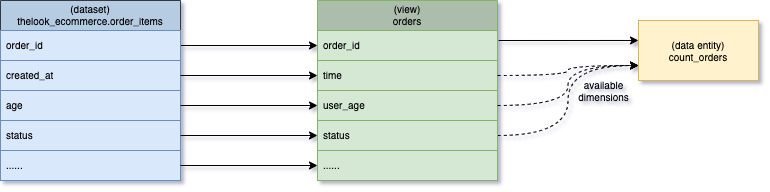
As shown above, the solid arrow represents the source lineage from the source field to the target field, while the dashed arrow implies that all dimensions from the view are available to the consumer when they consume the data entity with filters and group bys.
Lineage in Action: Detect Breaking Changes
Now, let's look at two quick examples of lineage in action, where it can be used to detect changes that may negatively impact downstream consumers.
Changes in Single Origin
Users are able to modify views, dimensions, and data entities in Single Origin, which can impact downstream consumers like reports, dashboards, or ML models. To prevent breaking changes and avoid the massive headaches that come with them, Single Origin leverages field-level lineage graphs to detect and monitor breaking changes automatically.
Changes in your Data Warehouse
When a dataset schema is changed (when a column is dropped, for example, or when a data type is changed) Single Origin can detect this and automatically check the updated field's lineage to determine if there is a downstream impact. Without this foresight, there can be unexpected consequences like incomplete or incorrect metrics for models and business consumers.
What’s next
We're excited to announce field-level lineage in Single Origin and look forward to developing the feature further to power new solutions for your organization. We can see a few potential use cases, including:
Policy Propagation
A policy applied to one entity can be propagated downstream to ensure policies between different entity types are inherited and consistent.
Automated Data Quality Debugging
Pinpoint exact upstream issues automatically when downstream usage has quality issues.
There are many more we can do with field-level lineage. Check back soon for our future updates. As always, feel free to reach out with any feedback or questions!