SQL Patterns (and how to exploit them) Part I

This blog is part one of our series, SQL Patterns (and how to exploit them). In this series, we will explore increasingly complex patterns that commonly occur in SQL and how Single Origin can exploit those patterns to consolidate and reuse SQL queries - saving users time and money. Check out our website if you want to learn more about Single Origin.

Today, it is impossible for data organizations to scale without sacrificing simplicity. The complexity of queries, pipelines, and infrastructure tends to grow exponentially. Meanwhile, the ability to detect duplicate work and reduce redundancies fades away. Additionally, metrics and definitions used by data and business operators can become difficult to discern and share.

Single Origin brings simplicity to the chaos through its semantic management platform. Semantic management as a term may seem broad, so in today’s article, we’ll focus on its potential impact on two data operators in the field. Each will be given a task and will write a query. Their queries contain a commonplace pattern that Single Origin can detect, and armed with this knowledge, our data operators will be able to reduce the complexity of their operations and improve the reusability of their SQL.

The Problem

Meet Jan and Michael - they work on the analytics team at Big Datum Incorporated. It’s Jan’s first day as a Data Analyst on the Promotions team, and she’s been given her first assignment. Jan’s boss wants her to build a dashboard that computes the per-customer coupon amount and net profit for:

• all out of town customers
• buying from stores in 5 cities
• over the weekend
• across three consecutive years.

Michael, a seasoned professional as a Senior Data Analyst on the Sales team, has a recurring task to generate an analysis report that is similar but distinct. He must compute the per-customer extended sales price, extended list price, and extended tax for the same segment of customers.

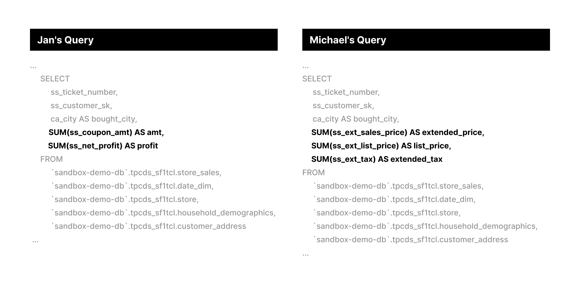
Working independently, Jan and Michael come up with the following two queries:

Jan and Michael’s queries may look familiar: they are from the tpc-ds, a well-known benchmark for big data analysis.

The Pattern

On inspection, you can see that the above queries share the same FROM, WHERE, GROUP BY, and ORDER BY clauses. Where they differ is what they are selecting. This pattern, where there is a difference in the selection, is commonly found in organizations writing lots of SQL.

SQL is a flexible language with no fixed style guide. So while the above example may be easy to notice, Michael could write an equivalent SQL statement with differing syntax. For example, Michael’s 62-line query without CTEs could be re-written as a 91-line query with CTEs. This would make detecting similarities more difficult for human reviewers.

Ultimately, the two queries are similar and, crucially, will generate duplicative work. Despite this, Jan and Michael fail to recognize the overlap. They don't review each other's SQL queries - they're on different teams after all. Even if they did, would they realize how to benefit from the similarities? Unfortunately, the two analysts write their queries in isolation. Their queries live on, perhaps used in an ETL pipeline or periodical query job. Jan and Michael never leverage the fact that they can utilize the same logic, and Big Datum is left to foot the bill.

That's where Single Origin comes in.

The Solution

Single Origin connects to your data warehouse and ingests your queries. Queries are then automatically decomposed, unlocking the following benefits:

• Pattern detection: Single Origin can detect patterns in queries across users, even when the query structure is completely different. This information is used to prevent duplicate logic.
• Reusability: Each piece of the query is defined and discoverable. This allows users to utilize components of prior queries. Single Origin can even re-construct one query from the component pieces of multiple queries, allowing for extensibility.

Let's take another look at Jan and Michael's workflows, but they'll use Single Origin for duplication detection and SQL reusability this time.

Michael logs into Single Origin and imports his initial query. The query is cataloged, so when Jan imports her query, she is alerted that duplication is present. She can then reuse Michael's definition and build on top of it.

In this scenario, Single Origin can help Jan and Michael consolidate their two query jobs into one job, saving on compute and maintenance costs.

Notice that Jan and Michael have gone from managing individual queries to managing shared definitions. This paradigm shift enables Jan and Michael to collaborate more easily, move faster, and build more efficient queries. Big Datum Inc is one step closer to achieving simplicity.

There are more patterns Single Origin can detect and more ways to reuse their SQL. Next week, we'll look at a more complex pattern. In our final post of the series, we will explore the ways Single Origin will leverage this technology in the future to deliver high-impact solutions for data operators and organizations at scale. So stay tuned!

For more articles, follow us on LinkedIn and subscribe to our blog! If you’re interested in learning more about the Single Origin platform, check out our website. For deep dives into how Single Origin’s SQL processing engine works, check out this series.

Until next time!