How Semantic Management can reduce your overhead and cut query costs by 50-90%

This blog explores a common pattern that occurs in ad-hoc SQL queries, and how Single Origin’s semantic management platform can exploit this pattern to save users time and money. If you’d like to learn more about Single Origin, you can visit our website.

TL;DR

We conducted a case study using a standard benchmarking dataset, and found that refactoring SQL queries based on patterns identified by Single Origin improved execution speed and costs by 50-90%. In one scenario provided below, we estimate thousands of dollars of savings from rewriting just three queries.

Introduction

Organizations face a growing number of challenges when scaling their data operations. In our last post, we detailed how Single Origin leverages SQL patterns to save organizations time by unlocking collaboration and reducing duplicative work.

In this post, we will dig into a SQL pattern that Single Origin leverages to identify query redundancies across an organization. Then, we will walk through methods for refactoring those redundancies to dramatically reduce cost per query and time to execute.

The Pattern

In large organizations there are a few patterns that can reveal underlying redundancies and inefficiencies across company data pipelines. One of the most common patterns arises from cross-departmental querying of different business metrics with different segmentations, but common source tables.

For example, there might be a growth team that has a dashboard for profit by state, while a sales team may have a dashboard of quantity sold by item ID. Instead of repeatedly querying against large tables, why not compute a simpler, consolidated view and query? Insight into where this pattern occurs in your ad-hoc queries can pave the way to optimizations that save big on performance and cost. That’s where Single Origin comes in. Single Origin identifies queries with common (reusable) logic and provides key insights so that users can better optimize both their data pipelines and ad-hoc queries.

At a high level, these are the two main ways that such insights provide value to users:

1. If Single Origin detects redundancy in queries that you run as part of a pipeline, then you may be able to remove some of your pipelines. When you remove pipelines, you save money (by not having to execute so many queries and store redundant results) and time (by not having to maintain/update/search more code). The savings comes from running fewer queries.
2. If Single Origin detects that there is redundancy in ad-hoc queries that are being run, then you may be able to pre-aggregate common, expensive requests. For example, if multiple operators are joining large raw event tables looking for similar things, then you may be able to run this large join and apply the necessary aggregations once a day and have operators query the output. While this could add one pipeline (so you are not running fewer queries), a lot of expensive queries run by operators become much cheaper.

Case Study

First, we needed to find a representative set of queries and datasets to audit. To this end, we landed on the benchmarking queries of TPC-DS. Next, we needed an engine to run the queries in, to establish a base cost and time to execute. We chose Snowflake, as they host the TPC-DS datasets for benchmarking purposes.  For the purposes of this case study, we limited the TPC-DS queries to target data from the year 1998.

Procedure

1. Run the benchmark ad-hoc queries in Snowflake and record the resulting cost and time to execute.
2. Run a Single Origin query audit on the benchmark ad-hoc query set to detect similar and duplicate queries.
3. Identify patterns to exploit in one of the groups of similar queries.
4. Leverage the pattern by writing a SQL pipeline capable of serving a pre-calculated table to optimize the benchmark ad-hoc SQL queries.
5. Run the rewritten benchmark ad-hoc queries in Snowflake, utilizing the SQL pipeline.
6. Compare the results of the initial query set to the results of the Single Origin optimized query set.
   

Single Origin Query Audit Results

In the TPC-DS query set, we found 15 groups of queries that fell into the pattern of common source tables but different segmentations. Each group had a few queries from the same source but with different selections, filters and group bys. We identified three queries that could be refactored to rely on a single pipeline to improve performance: queries 17, 25, and 29. For this benchmark, we will focus on the cost and performance of these three queries and their optimized counterparts.

Pipeline Generation

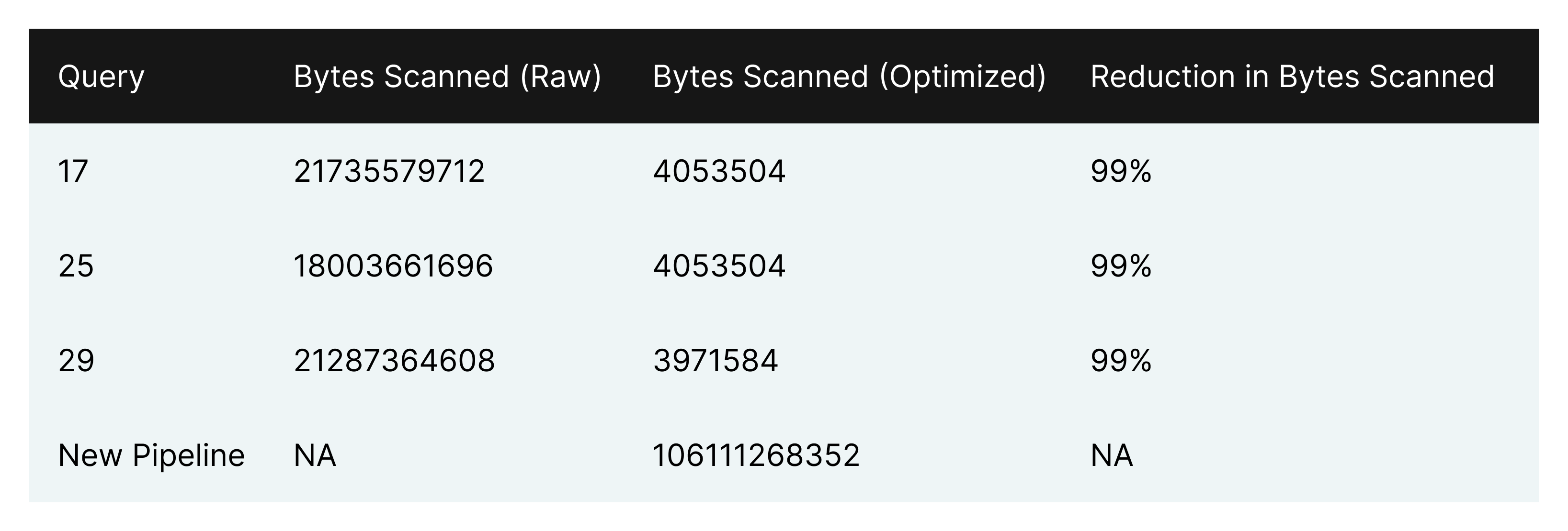
To maximize the performance of the three ad-hoc queries, we first generated a pipeline that could provide a common table to query against. Single Origin identified and extracted the common sources of the three queries - 8 inner join tables. These served as the pipeline’s source. Then, we combined the select, where and group-by clauses from the three queries and added them into the pipeline.

Optimizations

Based on Single Origin’s Audit Results, we performed a series of query optimizations. For each query, we replaced the source tables with the pipeline’s output. We also kept the original group bys to further aggregate the data from the pipeline output to calculate the original average and count aggregation values. For example, in query 17, AVG(SS_QUANTITY) is rewritten as SUM(STORE_SALES_QUANTITYSUM) / SUM(STORE_SALES_QUANTITYCOUNT), where STORE_SALES_QUANTITYSUM and STORE_SALES_QUANTITYCOUNT are aggregations provided by the new pipeline’s output.

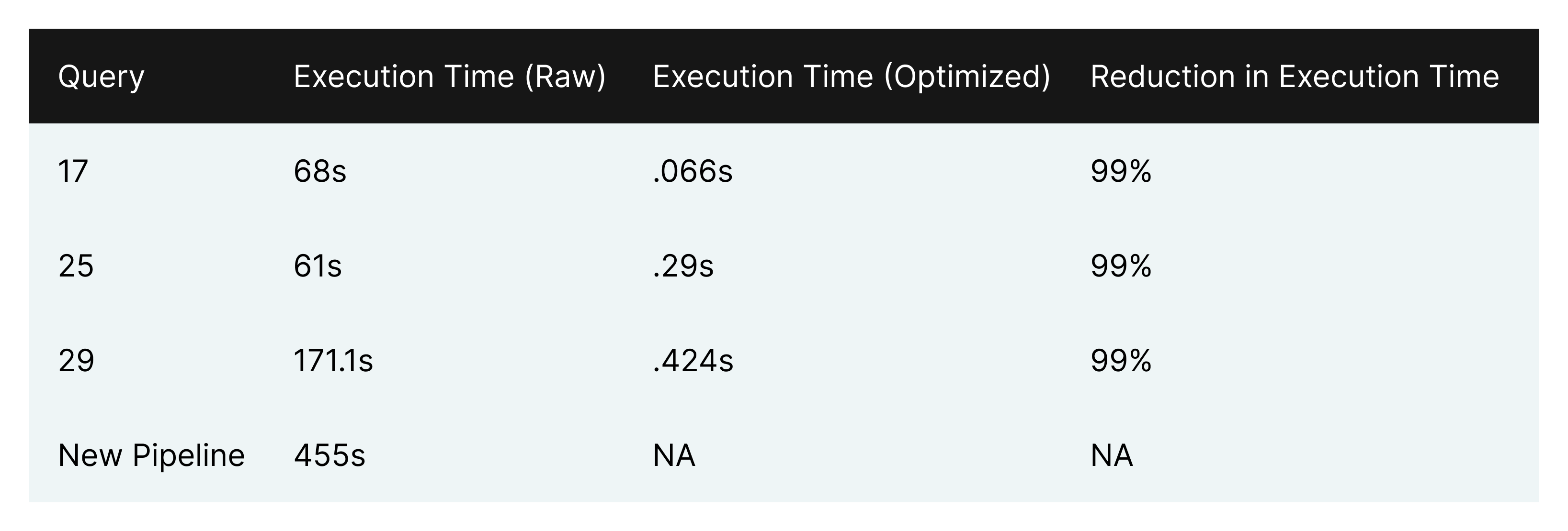
The resulting performance improvements for the ad-hoc queries were considerable.

Conclusion

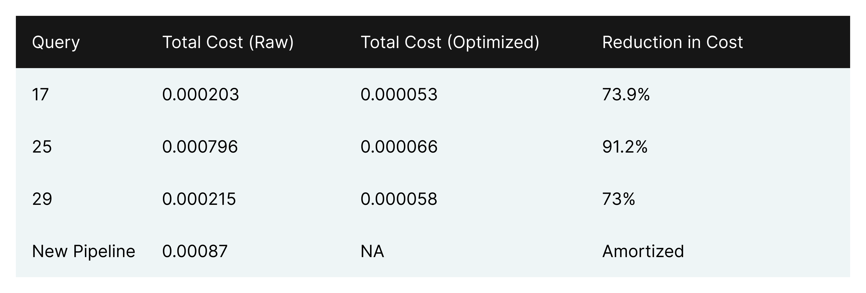
With the new SQL pipeline in place, the time for ad-hoc queries to execute was over 10 times smaller. By materializing a smaller table once a day that numerous queries can reference, end users are able to save a significant amount of time and money generating the same results as before. The other notable improvement was in cost. Before, one run of each ad-hoc query totaled 0.001214 credits (0.2c - 0.4c), whereas the cost of one run of each rewritten query was 0.000177 credits (.03c - .07c).

To give more tangible numbers, we can look at an example of a mid-size company, with 100 data operators. Of those 100 data operators, 25 of them run the above three queries 5 times a day, slicing and dicing the data. Over the course of a year, they will have executed the three queries 45,625 times. Before a pipeline is introduced, this would cost between $9,000 - $18,250 a year.

Now, we introduce our new pipeline to the equation. For this example, we will assume the pipeline is re-run three times a day (it is worth noting this would not hold for streaming data or real-time analytics). At three times a day, the same 45,625 ad-hoc query runs would run, in addition to 1,095 pipeline runs. The total cost in this scenario would be $1,370 to $2,880. This results in the organization reducing the cost of queries by between 68% and 92%. With insight from Single Origin and a few steps of refactoring, we significantly improved the performance and cost of the ad-hoc queries.

To realize the above savings without Single Origin, a user would have to sort through and analyze hundreds of queries (with differing structures), group them according to their similarities, and then start to refactor. Single Origin does this automatically.

Query auditing is just one facet of how Single Origin equips data teams with the knowledge and insight they need to make better decisions about their queries and pipelines. When queries are imported into Single Origin, the filters and group bys are stripped away, and any shared entities with the same source are deduped through the query import process. What you end up with, is one view and one data entity. When someone goes to query the data entity, they can plug in different filters and group bys. With this approach, definitions stay in sync, increasing data quality and unlocking collaboration across teams.

Single Origin also provides field-level lineage for your datasets, making governance and auditing easier than ever. Simply explore the lineage of your data to see who is accessing it and where it’s being consumed.

It is worth noting that there are many factors that influence performance and cost, including the complexity of your pipelines and the size of tables being queried.

While the cost savings in this case study required human intervention for refactoring, in the future this process can be automated because of Single Origin’s semantic understanding of your SQL logic. With this understanding, Single Origin could automate a lot of currently manual decisions:

• optimize your compute by organizing and running your pipelines based on their semantic lineage, as well as
• identify common query patterns and automatically add the underlying aggregation to your pipelines. This automates the existing loop of figuring out what pipelines to build based on what people care about.

If you’re interested in how Single Origin can help you compress your data pipelines and rewrite your SQL to optimize for cost and performance, reach out to us at support@singleorigin.tech.

Appendix

1.

Query 17

Rewritten query 17

Query 25

Rewritten query 25

Query 29

Rewritten query 29

New SQL pipeline